[This paper was published in the special 2003 polyhedra issue of the Symmetry: Culture and Science journal]
Stella: Polyhedron Navigator

Great Stella home page |
Robert Webb
Melbourne, Australia |

traduction en FRANÇAIS |
Abstract
We introduce Stella, a computer program for navigating the world of polyhedra. The user starts by choosing from a long list of built-in models, then uses advanced functions such as stellation, faceting, augmentation and excavation to explore the trillions of other possibilities. The symmetry group of any model is established and symmetries can be displayed. Nets for the physical construction of any model discovered can be printed out. Models may also be morphed into their duals in real-time on the computer screen, using one of five different techniques. In order to explain the concepts involved, this paper also represents a whirlwind tour of some of the major ideas in polyhedral theory today.
 Fig 1. Screen shot from Great Stella
 |
Many polyhedra are beautiful to behold. The mind is kept busy trying to grasp the various relationships that may exist in any given model. Polyhedra are a great example of a connection between art, craft and mathematics. However, the level of maths and draftsmanship required to build many models makes it somewhat prohibitive as a hobby for the less mathematically minded, and adds a considerable amount of time to the construction of any given model. Some simple polyhedra, such as the Platonic and Archimedean solids, pose no great challenge, since their faces are regular polygons which do not intersect. But the other uniform polyhedra, their duals, and stellations are more challenging. Measurements for some of these models are available on the internet or in books, most notably Wenninger's wonderful "Polyhedron Models" [28] and "Dual Models" [29], but a lot of work is still left to the reader, especially in the latter book (and since the calculations were done by hand, there are even some errors in the more complicated polyhedra).
Using a computer can make life easier. In this paper we present a computer program called Great Stella [27], or Stella for short, which allows the user to explore a great many polyhedra and print out the nets required for their physical construction. This eliminates the need for the user to perform tricky calculations, which are time consuming and error prone. It also removes the need to draft the various nets, which is also time consuming and prone to accumulation of inaccuracies. All that remains is the craft of scoring the edges, cutting out the pieces, and gluing them together. This automation brings the craft of making polyhedron models to a much wider audience.
Whether or not the user is interested in building physical models of their own, Stella lets them create and visualise models on the computer screen. The program allows the user to browse through a huge set of polyhedra and rotate them on the screen in real-time. All the uniform polyhedra are available through the list of built-in models. This set consists of the familiar Platonic, Archimedean and Kepler-Poinsot solids, an infinite array of prisms and antiprisms, and fifty-three other non convex polyhedra. The set, first described in its entirety by Coxeter and al. in 1954 [2], is very popular for its attractiveness (see figure 2 for an example). Skilling proved the set to be complete in 1975 [22], and introduced one new model which is also uniform, but doesn't quite classify as a true polyhedron due to more than two faces meeting at some edges. Skilling's new model is also built into Stella. The Johnson solids [10] (all convex non-uniform regular-faced polyhedra), many Stewart Toroids [25] (regular-faced non-intersecting polyhedra with genus greater than zero), and other models are also available from the list of built-in polyhedra. The program can also generate duals of all these models (see section 2), and the user has an array of polyhedral tools at their disposal for creating new models.
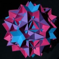 Fig 2. Great rhombicosidodecahedron
 |
Tools such as stellation, faceting, augmentation and drilling increase the set of available polyhedra tremendously, and open up an avenue for creativity in the discovery of new models. A number of research papers and books have been published on stellation theory ([1], [6], [7], [8], [14], [16], [17], [20], [21], [23]), and Wenninger's books ([28], [29]) also presented a collection of stellated polyhedra. Stella represents the culmination of all this theory, and can be used to produce most of the models presented in these publications, and many more. Faceting is another very powerful tool, but has not appeared much in the literature to date ([3], [9]).
Figure 1 shows what the program looks like. The big window on the left shows the compound of five tetrahedra, a stellation of the icosahedron. The smaller windows show one of the nets required top left, the icosahedron itself top right, the stellation pattern bottom left, and the cell diagram bottom right (these terms are discussed in more detail below). The window layout is configurable.
All the images with black backgrounds in this paper are photographs of models made by the author using nets printed by Stella. Nets were printed directly onto the colored paper used for construction. All other images were also created using Stella. The program runs on Windows 95/98/ME/NT/2000/XP. It has also been successfully used on a Mac via the Virtual PC Windows emulator.
In section 2 of this paper we explain the concept of duals. In section 3 we describe the process of stellation and some of the theory behind it. Section 4 explains the creation and printing of nets and how stellation theory can help. Section 5 discusses faceting, the dual process of stellation. Section 6 covers augmentation, excavation and drilling. Section 7 deals with symmetry, and how sub-symmetry can be used in conjunction with the previously described operations. Section 8 presents our techniques for morphing between dual models. And finally, in section 9 we will examine some additional capabilities not already covered.
For any polyhedron, there exists another polyhedron which is its dual. Taking the dual of this dual polyhedron returns us to the original polyhedron again. Roughly speaking, vertices are replaced with faces, faces with vertices, and edges with new edges orthogonal to the originals.
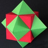 Fig 3. Compound of cube and octahedron
 |
More precisely, the technique used to create a dual is spherical reciprocation. This is done with respect to some sphere, and the choice of sphere affects the resulting dual polyhedron. Typically the center of the sphere is placed at the center of symmetry, if one exists (where all the axes of rotational symmetry or planes of reflective symmetry intersect). The radius of the sphere is usually the midradius of the polyhedron, if one exists (the radius of a sphere touching all edges of the model tangentially). Stella will choose an appropriate sphere for the operation.
Let's suppose r is the radius of the sphere to be used, and C its center. If the distance from a face plane to C is d, then the distance from C to the corresponding dual vertex is r2/d. Similarly, if the distance from a vertex to C is d, then the distance from C to the plane containing the corresponding dual face is again r2/d. Additionally, the direction from C to the dual face plane or dual vertex is the same as the direction from C to the corresponding original vertex or face plane.
We refer above to the face plane rather than just the face because the distance from C should be measured to the closest point in the face's plane, which may indeed be outside the face.
From these simple formulæ, the vertices and faces of the dual model may be obtained. Note that multiple faces in the same plane will all be mapped to the same dual vertex position. Note also that if a face passes through the center of the sphere, its dual vertex will be at infinity, since the distance to that vertex will be based on division by d which is zero.
Stella allows the user to view a polyhedron and its dual at the same time in separate windows. It may also display a compound of the two. For example, the cube and octahedron are duals. Their compound is shown in figure 3. Nets for the physical construction of these compounds are also available within Stella.
3.1. What is a stellation?
The act of stellation opens up an almost endless collection of fascinating models. The number of stellations of a single polyhedron will often be measured in the trillions. The most general definition of the term says that two polyhedra are stellations of each other if their faces lie in the same set of planes. The exact definition has been somewhat debated, but the author believes all other definitions are subsets of that which is given here. More justification for this definition will be given below, but first, a little more theory is required.
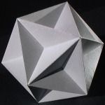 Fig 4. Great dodecahedron
 |
Sometimes several stellations may appear to be identical. For example, consider the great dodecahedron, which is a stellation of the dodecahedron, and consists of 12 intersecting pentagons (see figure 4). When observing this model, part of each pentagon is hidden from view, internal to the solid. As a result, only five triangular regions are visible from each pentagon, so the model could also be thought of as comprising only those visible triangles. The polyhedron would then have 60 triangular faces, and no hidden parts. There are also other polyhedra that appear identical to the great dodecahedron from outside. However, within any set of stellations that are identical in appearance, there is always exactly one that consists only of the parts that are visible, or rather accessible, from outside. The stellations created in Stella are of this form, but otherwise there is no restriction on what stellations can be made, (except that they must be finite). For example, if the user were to create the great dodecahedron as a stellation of the dodecahedron, the model they would get would really consist of 60 triangular faces, not 12 pentagons, but would otherwise be identical in appearance to the true great dodecahedron. It is important to recognize however that the two polyhedra are indeed different. If the user wishes to distinguish between multiple possibilities, faceting can be used (see section 5).
So how do we find the stellations of a polyhedron? Each face of the polyhedron lies in some plane. We can think of each of these planes as carving up space, partitioning it into a collection of three-dimensional convex cells. The first plane divides space into two parts, the second divides each of these parts in two giving us four parts (unless it is parallel to the first plane), and similarly, the third gives us seven or eight parts. All these parts are infinite though, that is, none of the parts are entirely bounded by planes yet. Once we add the fourth plane things get more interesting, as now there is one finite cell, bounded by planes on all sides. This is the situation when stellating the tetrahedron. The only cell that is finite is the tetrahedron itself, and so there are no other stellations.
The dodecahedron is a more interesting case. Its 12 faces lie in 12 planes, which carve up space into 63 finite cells. Due to the symmetry of the original polyhedron, the cells fall into symmetric sets, referred to as cell types. The 63 cells fall into four cell types. The dodecahedron itself is the central cell, and the only one of its type (see figure 5a). The next type consists of 12 pentagonal pyramid cells, which sit on each face of the dodecahedron, giving rise to the small stellated dodecahedron (see figure 5b). Next are 30 tetrahedral wedges, which fit between the spikes of the previous model and form the great dodecahedron (see figure 5c). And finally, 20 dipyramids fit into the dimples of the great dodecahedron to form the great stellated dodecahedron (see figure 5d). We construct different stellations by including different combinations of cell types. A stellation is usually required to have the same rotational symmetry as the original polyhedron, so we either include all cells of a type, or none. For this reason the two are synonymous for most purposes, and from here on we shall refer to cell types simply as cells.
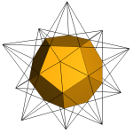 Fig 5a.
 |
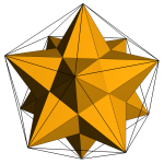 Fig 5b.
 |
 Fig 5c.
 |
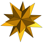 Fig 5d.
 |
|
Fig 5. Stellations of the dodecahedron, adding one cell at a time, and showing where the next cell will go in wire-frame |
The stellation process performed by Stella is extremely fast when compared with some other programs that perform stellation, taking less than a single second for any uniform polyhedron or one of their duals on an average machine, where other programs might take many minutes or far worse. Internally, Stella starts by generating the 2D stellation diagrams (see section 3.3). This takes great advantage of the model's symmetry by only creating diagrams for one of each face type, and also reduces the task from 3D to 2D, where calculations can be done more efficiently. Both of these aspects save greatly on the time and memory required. Cells are then created as sets of the elementary regions that enclose them. Again, data is only required for each cell type rather than each individual cell. Other approaches have started by generating the geometry for every individual cell, then grouping them into cell types and generating stellation diagrams. These approaches are more straightforward, but much less efficient.
3.2. So what is a stellation really?
As stated earlier, there has recently been some debate as to how "stellation" should be defined. In this paper we say that two polyhedra can be stellations of each other. So, for example, it could be said that the dodecahedron is in fact a stellation of the great dodecahedron. However, in Regular Polytopes [3], Coxeter refers to extending faces until they meet again, which conveys the impression that the stellation process can only go outwards. Even the term itself means to turn into a star, and has an emotive quality, conjuring up images of pointy objects with sharp spikes. So is our definition inconsistent with the existing literature?
One idea few previous publications have addressed is stellation of non convex polyhedra. It could simply be disallowed, but we see no justifiable reason for that. Stellation is really an operation for which the input is a set of planes. The planes usually come from face planes of a given polyhedron, but there is no obvious reason to restrict the polyhedron to being convex (or even to require that the planes be derived from a polyhedron at all!). The set of planes can be used to generate all the possible models with faces in those planes, and we refer to these models as stellations. This is the basic operation being performed. It would be a seemingly pointless restriction to only allow those stellations that were "extended" with respect to the original polyhedron, whatever that means exactly.
Of course, in "The Fifty-Nine Icosahedra" [1], Coxeter included hollow stellations of the icosahedron, where the faces of the original icosahedron were no longer present. This may also seem to go against the idea of "extending faces", but the important point is that the face planes are still present. If those models were not considered stellations of the icosahedron, then what are they stellations of? Or, is this another case for which we draw an arbitrary line and disallow stellation altogether? Previous literature has used whatever terminology was relevant at the time. "Regular Polytopes" was not interested in stellation for any purpose other than how it related to regular polytopes (in three dimensions, a polytope is just a polyhedron), so it was appropriate in that case to simply refer to "extending faces", since they would not be dealing with hollow polyhedra and other such cases. More generally, terminology has reflected the fact that various authors have only considered stellation of a convex core. Stellations were always "extended" in a sense because when starting with a convex polyhedron, one could not get any smaller.
In this paper we extend the definition to allow stellation of non convex polyhedra, and freely allow those stellations to be smaller or bigger than the original. Thus we must include the convex core as one such stellation. This definition does not contradict any previously published works, it merely takes the concept to its natural conclusion. Often as a scientific field expands, old ideas are applied to new situations that were previously not considered. The old ideas must then be updated accordingly. The important thing is that the updated concept still behaves as always in the original situations, and has a natural extension to new situations.
Maybe the emotive term "stellation" doesn't always seem quite right anymore, but it still sounds right in most cases, and it would be unwise to change it now. Many traditional stellations do not look like stars anyway.
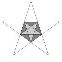 Fig 6a. Dodecahedron
 |
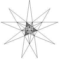 Fig 6b. Icosahedron
 |
|
|
Fig 6. Stellation diagrams |
There are two important concepts in stellation theory: the stellation diagram and the cell diagram. Both of these can be displayed within Stella. The stellation diagram (see figure 6) is a two-dimensional diagram that lies in the same plane as one of the faces of the original polyhedron, and shows a line for each intersection with one of the other face planes. The lines enclose finite areas known as elementary regions [17]. Infinite areas, i.e. those not completely enclosed by lines, are left out, and any part of a line that does not have a finite elementary region on at least one side is not shown. One stellation diagram is required for each type of face. For example, only one diagram is required for the icosahedron, as all faces share the same relationship to the whole.
Any stellation can be specified by filling in a collection
of elementary regions to represent the externally accessible parts of that stellation. Figure 6a shows regions required for the great dodecahedron (a stellation of the dodecahedron, see figure 4). Figure 6b shows regions for the familiar compound of five tetrahedra (a stellation of the icosahedron, see figure 1). Dark shading shows the regions required, while lighter shading shows other regions that are internal to the solid. Stella uses different colors for the following four types of regions: regions that are accessible from above the plane, regions that are accessible from below the plane, regions that are internal to the model, and regions that are outside the model. This representation is more convenient than trying to specify the situation in 3D. Each elementary region has a cell above it and another cell below it, and represents a face of those cells. Stella allows the user to include or reject the cell above or below a region with a click of the mouse (as long as the cell is finite). The stellation diagram may be viewed flat in its own window, or displayed in 3D perspective attached to one of the faces of the original or stellated model, which gives the user a good feel for what the stellation diagram is all about.
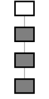 Fig 7a. Dodecahedron
 |
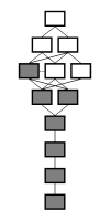 Fig 7b. Icosahedron
 |
|
| Fig 7. Cell diagrams |
The cell diagram (see figure 7) was first introduced by Messer [17], building on an earlier concept from Pawley [21]. Starting with the inner core, cells form layers, each completely obscuring the previous layer from view (with the exception that some cells in the outer layers may be infinite, and these are typically excluded, leaving gaps through to lower layers). A layer may contain one or more different cells (i.e. cell types). The cell diagram is a graph in which nodes represent cells. Cells in the same layer are drawn at the same height in the graph, with the innermost core cell at the bottom and the outermost layer at the top. Lines connect any two cells that share a face. Since each layer entirely covers the previous one, lines can only ever connect cells from two consecutive layers. Since we are usually interested in stellations with the same rotational symmetry as the original polyhedron, but not necessarily the same reflection symmetry, we ignore reflections when grouping cells into types. As a result there may be two nodes in the cell diagram that represent an enantiomorphic pair of cell types. Such pairs are always drawn side-by-side, with a dashed line connecting them. Other authors have usually represented these enantiomorphic pairs as a single node in the cell diagram, but we have found it more useful to separate them. As with the stellation diagram, some cells in the cell diagram can be filled to indicate their inclusion in a stellation, thus the cell diagram is also a convenient way to represent any particular stellation (the shading in figure 7 corresponds to the same stellations as in figure 6). Again, cells can be included or rejected from a stellation with a click of the mouse on a cell in the cell diagram.
In any situation in which a cell may be selected for inclusion in, or rejection from, a stellation, Stella's interface gives the user a few options about which cells to affect. The user can simply turn a single cell on or off, or turn a cell on or off along with all the cells that support it (that is, all cells that can be reached by starting at the selected cell and following a sequence of downward lines in the cell diagram). This makes setting up many stellations a lot quicker. The user can also choose to turn on or off all cells within the same layer as the selected cell.
The interface also has a button for filling-in
any inaccessible cells. In some cases the user may have designed the stellation that they want, but may have left bubbles inside where cells are not included, leaving hollow parts that cannot be accessed from outside. This function automatically includes such cells. For a user planning to print out nets for the construction of a physical model, it is a good idea to use this filling-in function first, otherwise nets for the inaccessible parts hidden inside the model will also be printed.
 Fig 8. Stellation of small stellated truncated dodecahedron
|
Various investigators have proposed restrictive rules, both to reduce the number of stellations to more manageable sets, and to avoid "uninteresting" cases. As an alternative to manually selecting which cells are required for a particular stellation, Stella also supports various sets of rules, allowing the user to choose a set of rules, and step forward or backward through the list of all stellations satisfying those rules for any model. This provides an easy way to browse through many interesting stellations without having to manually select or deselect cells. The following five sets of rules for choosing stellations are supported in Stella.
-
The first and best-known set of rules was proposed by Miller in "The Fifty-Nine Icosahedra" by Coxeter and al. [1], and these criteria have become known as Miller's rules. There are five rules. The first three simply cover the definition of stellation and ensure that the stellated model has the same rotational symmetry as the model being stellated. The fourth rule requires that all 2D elementary regions used for the surface of the stellation are accessible from outside the model. And the fifth rule requires that the model is not a compound of two other stellations satisfying these rules, each with as much symmetry as the complete stellation.
By Miller's rules there are 59 stellations of the icosahedron, which includes the original icosahedron itself in the series (as will be done for all counts hereafter). These rules allow some models with holes through them, and even with completely disconnected parts. As with Stella, Coxeter and al. found stellations by only considering the externally accessible parts, thus leaving out multiple stellations that looked the same from outside.
-
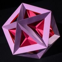 Fig 9. Stellation of great stellated truncated dodecahedron
 |
For models more complicated than the icosahedron, Miller's rules quickly lead to a very large number of stellations. In 1975 Pawley examined stellations of the rhombic triacontahedron [21], and employed different criteria for accepting stellations, thus reducing the set to a more manageable size. He called these non-reentrant stellations, now known better as fully supported stellations [17]. These are all the stellations for which any ray from the center outwards will only ever cross the surface once. So models with holes or over-hanging parts are no longer included. The stellations found are a subset of those found using Miller's rules. The term fully supported comes from an observation of the cell diagram (see section 3.4) for such models. Any cell reached by following a line downwards from a used cell must also be used in a fully supported stellation, thus each cell is fully supported by all cells below it. There are 18 fully supported stellations in the series for the icosahedron.
-
The number of fully supported stellations for some polyhedra also becomes prohibitively large. Mainline stellations is a far more restrictive set. A whole layer of cells must be added in order to step from one of these to the next, starting from the central core cell. Mainline stellations are therefore a subset of the fully supported stellations. The number of mainline stellations is therefore simply the number of cell layers; eight in the case of the icosahedron. For more complex cores, the mainline stellations tend to look a little "messy", so although the set is reduced, it is generally not reduced to only the most interesting models.
-
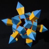 Fig 10. Stellation of dodecahemicosahedron
 |
A more restrictive, but also more interesting set, is the set of primary stellations. Primary stellations were introduced by Messer in 1989 [16]. However, the set is only well defined for reflexible isohedral cores, such as the platonic solids and the Archimedean duals (aka Catalan solids). Primary lines in a stellation diagram are those that lie in a reflection plane. These lines can be highlighted in Stella. A primary region is an area of the stellation diagram that is enclosed on all sides by primary lines, with no other primary lines crossing the area. The face of a primary stellation is simply one primary region. Every primary region leads to a valid stellation. This set is another subset of the fully supported stellations, but the resulting models are far more appealing. Given that these stellations are always isohedra (that is, only having one face type), they never look too messy. This is in fact the most restrictive set generally, as there is only one stellation included for each primary region, and the number of primary regions is limited by the order of the symmetry group. For the icosahedron, there are seven primary stellations in the series.
-
Another interesting set was also proposed by Messer (unpublished, but introduced here with kind permission), which he calls monoacral, meaning single peak. This is another fairly restrictive set, and another subset of the fully supported stellations. To make a monoacral stellation, start with any single seed cell and make the minimal fully supported stellation which includes that cell. This can be achieved by adding all the cells required to support the seed cell, and all the cells required to support those cells, and so on down to the central core.
3.7. Extended stellations
In 1989, Fleurent described the concept of an extended stellation diagram [7]. This is the stellation diagram obtained when stellating the compound model consisting of a chiral polyhedron and its enantiomorph (mirror image). Stella has a built-in function to create such a compound from any chiral polyhedron, after which the standard stellation process can be applied.
3.8. Stellation examples
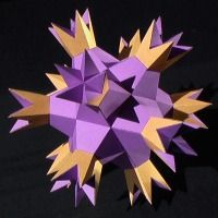 Fig 11. Stellation of dodecahemicosahedron
 |
A model does not have to be convex to be stellated. All the process of stellation really requires is a set of planes, which come from the faces of a given polyhedron. Hudson and Kingston [8] presented a number of stellations of non convex uniform polyhedra, but otherwise there has been little mention of the idea in the literature. Nevertheless, some beautiful stellations exist of non convex polyhedra. Figure 8 shows a glorious stellation of the small stellated truncated dodecahedron. Figure 9 shows a very Zen stellation of the great stellated truncated dodecahedron. And figures 10 and 11 show stellations of the small (or great) dodecahemicosahedron.
Nets are the externally accessible parts of a model, separated from each other at some edges, where necessary, so that they may be folded flat (see figure 12). They can then be drawn or printed on paper, cut out, folded, and glued to reconstruct the model. Two steps are required for the automatic generation of good nets. First, the externally accessible parts must be identified. And second, those parts should be combined, where possible, in order to form larger nets.
For the physical construction of a model, the author uses and recommends the double tabs method, as described by Wenninger [28]. This method involves leaving tabs on all free edges around each net. Pieces are then connected at an edge by gluing the two tabs together at that edge, which leaves a kind of ribbing inside the model. This method produces high quality models, and clamping tabs together is easily achieved with a pair of tweezers.
4.1. Identifying the parts
The stellation process and construction of nets are closely related. As described above, a stellated model in Stella consists only of its externally accessible parts, which happens to be exactly what we need for creating nets. A model builder will generally not wish to make the parts of faces that are hidden inside a model (one notable exception is Ulrich Mikloweit [18], who cuts artistic designs into his faces, making the internal parts visible again!). So the elementary regions used by a given stellation are exactly the parts required for the nets. This shows the usefulness of stellation, whether or not someone is interested in the stellated polyhedra themselves.
This is fine for a model discovered via stellation, but what about a uniform polyhedron, or one of the others from the built-in list, or a faceted polyhedron (see section 5), or any other polyhedron derived using a technique other than stellation? First the user would have to stellate the model and figure out which stellation cells are required to reproduce that model. Remember, the original model may have intersecting faces with parts hidden from view, whereas the stellated version will consist only of the externally accessible parts required for generating nets. Selecting the appropriate cells manually can be a tedious task for complex models.
Again, Stella automates this process. When a new model is created (either chosen from the list, or generated using tools such as faceting), and nets are required, the stellation process is performed first, and the appropriate set of cells is automatically selected to reproduce the original model. This is a tricky task, requiring an algorithm that spreads across the exterior of the model, keeping track of which way is "up" and selecting any cells below the surface as it goes. Any inaccessible cells are then filled-in, as described in section 3.5. Note that for different parts of the same face, the cell above, below, or both could be required. To the best of the author's knowledge, no other program can currently perform this task.
4.2. Combining parts into nets
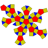 Fig 12. Net of rhombicosidodecahedron
 |
Once the required parts have been identified, an attempt is made to combine them together, where possible, into larger nets. By combining two parts which share an edge into a single net, the model maker need only score and fold that edge once, rather than cutting out the edge for both parts, generally leaving a tab which also requires scoring and folding for both parts, and then gluing the tabs together. When lots of parts can be combined in this way, it can save the model maker a considerable amount of time. Stella does a good job in most cases of combining as many pieces as possible into single nets, using various heuristics to decide which parts should be combined in preference to other parts. Stella ensures, of course, that the parts never overlap within a net. Nets are created symmetrically and kept sorted into net types. A new part will not be added to a net unless it can be added symmetrically to all parts of that type. This generally leads to much nicer nets, and the model maker can get into an efficient routine when scoring, cutting and folding many copies of the same net.
At some edges parts must not be combined into a single net. For example, the user may choose to group only like-colored parts into any single net, and then to group like-colored nets when printing. This is useful in order to print the nets onto colored paper stock. The user would print all the red nets onto red paper first, say, and then separately print all the yellow nets onto yellow paper. This is the default mode in Stella, as the author finds this to be the most useful way to make models, and Stella knows not to combine parts of different colors in this case. When this mode is disabled, different colored parts will happily be combined, and the user may choose to use a color printer to fill in the color of each face, or to leave their interiors blank if they do not require any color or will decorate the parts themselves.
The user may also manually tell Stella to cut some edge, that is, to not combine nets at those edges. Stella will then regenerate the nets, possibly joining other parts together instead. This is useful if the user is not happy with the automatically generated nets, and wants to force other parts to combine instead, or wishes parts to be completely separate. There is also an option to set the maximum number of parts that may be combined into any one net, to prevent nets from becoming unmanageable. This value may also be set to "1" to force all the parts to remain separate, for example when using very thick card that can not be folded cleanly.
There is another situation that also requires special handling. Some models have coincident edges, where two solid sections meet each other only at an edge. The simplest of the uniform polyhedra, the tetrahemihexahedron, is an example of this. As in this example, the edge may not be a true edge of the model, but rather just the intersection of two faces as they pass through each other, but this makes no difference when constructing a model. The question is whether or not to combine parts into single nets at these edges. Firstly, it should be pointed out that there is actually an ambiguity regarding which parts would be combined, since four parts meet at the edge. But if parts are to be combined, it should be the parts that appear connected from outside the model, otherwise the two sections would not be connected to each other at all and the model would fall apart. The user has a choice for how to treat such edges. They can choose the tongue in groove method, as described by Wenninger [28], where the double tabs on one section are glued together pointing out rather than in, and the matching double tabs on the other section are left pointing in, but unglued. The former tab is then coated with glue and slotted between the latter tabs. This method requires tabs on all four parts, and hence no parts may be combined at this edge. Another option is the internal support method, where at least one of the pairs of parts must not be combined, so that a double tab is present. This tab is then glued internally behind one of the parts from the other pair, contributing to the rigidity of the model. In this case one of the pairs of parts may still be combined. This is generally the author's preference. Finally, the user may choose the no internal support required method, where both pairs of parts may be combined into single nets if possible. However, this method may lead to a less robust model, as there could remain some flexibility in the parts at such edges.
Finally, if the model is convex, then an attempt is made to connect all the parts into a single net.
4.3. Arrangement of nets on the page
In the interface, one net is shown on the screen at a time, and the user may step through all the different types of nets required to build the model. The interface indicates how many of each net are required for construction. When printing however, obviously all nets are printed together, and Stella tries to fit as many nets on each page as possible, for optimal printing efficiency. For each page, it starts with the largest net, trying to fit as many of them on the page as it can (up to the number required of course), then moves to the next biggest net and tries to fill in any remaining gaps, and so on. If the user has chosen to group like-colored nets together, then only nets of the same color will appear on the same page. On the final page, Stella also tries to leave as big a gap as possible at the bottom of the page, in case the user wants to use the space to start printing out nets for another model.
Stella gives the user control over the four margins of the page, so that they can make use of blank parts of an otherwise printed page by feeding the page back through the printer (be careful to put it in the right way around though!). There is also an option to set the top margin specifically for the first page, in case printing is to be continued from where the previously printed model left off. A convenient button sets this automatically to be just below the point on the page where the previous print out finished. This helps save paper, especially in cases where only a few small nets are printed on the final page, leaving the page otherwise blank.
The scale of any model can be set in a number of ways. This does not affect the appearance of the model in the interface. It only affects the size of the nets that are printed out, and any numerical measurements given. The scale can be specified by setting the radius of a stellation or its base model, or an edge length, or the distance between any two vertices. Users can also view and set the length of the shortest edge in the stellated model, which is useful because this is the smallest edge that will need to be cut out, and will be difficult to manage if too small. When printing, Stella will first check whether any nets are too big to fit on a page, and if necessary, give the option of automatically reducing the scale so that all nets just fit. The user may instead wish to force large nets to be broken into smaller nets, and then try printing again to see if the smaller nets now fit.
4.4. Data for alternative construction
Dihedral angles and edge lengths may be displayed on each edge in a net, and face angles are also available. This data is useful for the user who wants to draft their own nets, for example on material that would not fit through the printer, or construct models from wood, where edges of parts must be bevelled based on the dihedral angle between faces.
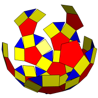 Fig 13. 3D folding net of rhombicosidodecahedron
 |
4.5. 3D folding nets
The nets may be viewed folding and unfolding in real-time in 3D (see figure 13). There are two halves to this process. Starting with the completed model, the individual nets are first spread out from each other (if there is more than one net), and then each net unfolds until flat. The spreading out is required to give the nets room to unfold. Sometimes they will still pass through each other when spreading or unfolding, but the effect is still impressive, and this feature can serve as a useful reference when building a model and trying to figure out how pieces fit together.
A facet of a given polyhedron, as we will use the term here, is a polygon whose vertices are also vertices of that polyhedron. Facets that lie entirely inside a model can be useful as internal struts to add support for physical models that may otherwise not hold their shape well. They are glued inside during construction, generally using the already glued double tabs from other external parts. Stella provides a mode for creating facets, which can then be printed out along with the other nets. The user clicks the mouse on each vertex of the facet in turn until the facet is complete (see figure 14), and then confirms acceptance of the facet or rejects it. After making about half a model, the builder can usually get an idea of how robust the result will be, and this is a good time to consider inserting some of these facets to add rigidity to the model.
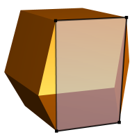 Fig 14. Rhombic dodecahedron showing a
user-defined rectangular facet |
Faceting is a very powerful tool that has had little exposure in the literature. It is the dual process of stellation, as discussed briefly in Coxeter's "Regular Polytopes" [3]. Inchbald [9] gives a more in-depth study of this relationship as it relates to the stellations of the icosahedron, and the dual facetings of the dodecahedron. Just as stellation may be defined as two models with faces in the same planes, faceting may be defined as two models with the same vertices. For example, the small stellated dodecahedron (figure 5b) is a faceted version of the icosahedron, and so are the great dodecahedron (figure 4) and the great icosahedron. The great stellated dodecahedron however (figure 5d) is a faceted version of the dodecahedron.
Wenninger describes an interesting relation in his book "Dual Models" [29], where he says:
|
the face of the dual of any non convex uniform polyhedron is embedded in the stellation pattern of the dual of its convex hull. |
The convex hull of a model is a special case of a faceting of that model, where the result is convex. Normally we would think of this the other way around, i.e. that the non convex model is a faceting of the convex one, but this general definition, which matches our general definition for stellation, works well in practice for situations like this. It should be pointed out however that the convex hull of an arbitrary polyhedron would not always be a true faceting, as some inner vertices may be lost, making it only a partial faceting. To generalize Wenninger's statement, if we take some faceting of a polyhedron and create its dual, then some stellation of this new model will be the dual of the original polyhedron. Choosing to take the convex hull is simply a special case of a faceting, and its dual will be a special case of stellation, namely the innermost core cell.
Conversely, if we take some stellation of a polyhedron and create its dual, then the original polyhedron is a faceted version of this new model. Similarly, we could again choose the special case of the only convex stellation, that is, the central core cell, which will give us a convex dual to be faceted. Hopefully this points out the duality of the stellation and faceting processes, and demonstrates that each must therefore be as powerful as the other.
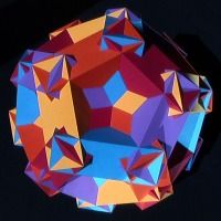 Fig 15. Compound of fifteen cuboids
 |
We previously explained how facets could be made in Stella for the purpose of adding robustness to physical models (see section 4.6). However, the user can also choose to create a new faceted polyhedron from the facets they have created. In this case, the facets are repeated over the symmetry group to produce all occurrences of each one. It is up to the user to make sure they have created a set of facets that will lead to a valid polyhedron where two faces meet at each vertex, and so this is a somewhat advanced feature requiring a certain amount of skill to use well, but it is also very powerful.
Some examples will serve well here. Figure 15 shows a faceted truncated dodecahedron. It is also a compound of fifteen cuboids (rectangular prisms). This model has three different face types, and so three facets of the truncated dodecahedron must first be defined. Stella can then repeat them over the symmetry group to create the whole model. As with any model, it can then be stellated, and nets can be printed out.
Here's another example. There are only four rectangular isohedra (polyhedra where all faces are rectangular and share the same relationship to the model as a whole). All are facetings of duals of uniform polyhedra, and so they can all be made using Stella. Figure 16 shows one such model, a faceting of the rhombic dodecahedron. Since there is only one face type, all that is required is clicking on the appropriate four vertices of the rhombic dodecahedron to create one facet (the facet required is shown in figure 14). Stella can then construct the whole model.
Users may stellate faceted models, and facet stellated models, which leads to an unthinkably large set of polyhedra. We referred above to one of the four rectangular isohedra. Two of the others (a faceting of the rhombic triacontahedron and a faceting of the great rhombic triacontahedron) happen to have the same stellation pattern as each other. This stellation pattern also happens to be the same as that of the compound of five dodecahedra described by Cundy and Wenninger [5] (see figure 17) and thus the compound of five great stellated dodecahedra which they also describe, and the compounds of five small stellated dodecahedra and five great dodecahedra introduced earlier by Smith [24] and shown in [19]. So these models can all be created, along with the dual compounds of five icosahedra and five great icosahedra. Many thanks to Piotr Pawlikowski who recently discovered this relationship between the rectangular isohedra and the five-dodecahedron compound. It is believed to be previously unpublished, and is used here with his kind permission.
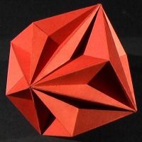 Fig 16. One of four rectangular isohedra
 |
Reference was made above to the fact that stellations in Stella consist only of the externally accessible parts, however, faceting can be used to specify the true model required. One good reason for wanting to do this is to acquire its proper dual. Although the stellated models may appear the same, their duals probably won't. In the previous example, the compound of five dodecahedra is obtained by stellation of another model, so the model consists only of the externally accessible parts rather than the intersecting regular pentagons that it should. But faceting can fix this. The user just needs to click on the five vertices of one of the pentagons and tell Stella to create a faceted polyhedron. Note that all pentagons in this model are of the same type (they each have the same relationship to the model as a whole), so only one facet need be created. Now we have the true model, and can see its true dual; the compound of five icosahedra (which can then be stellated of course to create a compound of five of any stellation of the icosahedron!).
Another set of intriguing models that can be investigated using a combination of stellation and faceting are the isogonal isohedra. These are polyhedra with only one type of face and only one type of vertex. Obviously the nine regular polyhedra (Platonic and Kepler-Poinsot) fall into this category, and there are some distorted tetrahedra that also fit, but there are also some other strange models. Three are stellations of the icosahedron, and two are stellations of the rhombic triacontahedron, including the final stellation of each. This amounts to five new models. The dual of any model in this set must also be an isogonal isohedron, since properties of vertices and faces are exchanged, which implies there should still be only one type of face and one type of vertex. This in turn brings the number of new models to nine, since one of the stellations of the icosahedron is self-dual. As an example, the final stellation of the icosahedron may be seen as having irregular enneagrams for faces, that is, nine-pointed stars. They meet by threes at each vertex. Stellation can be used in Stella to find the model, and then faceting can be used to specify how exactly the face should be constructed (that is, as an irregular enneagram). From here the dual model can also be found.
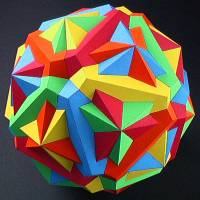 Fig 17. Compound of five dodecahedra
 |
For some interesting work with faceted models, have a look at the recent work of Klitzing [12]. He calls his models edge-facetings, as all the faceted models within a series share not just the same vertices, but also the same edges. He also restricts the facets to be regular polygons, but lifts the restriction that all vertices must be used in the faceted model. Stella should be able to make all these models.
There is currently one limitation that should be mentioned when creating facets, namely that the same vertex must not be visited twice within one facet. This is not a common situation, but is worth mentioning. Some models that have more than two faces meeting at an edge may also have problems. These are not true polyhedra, but many are interesting nonetheless. Most of these models will still work, for example Skilling's new uniform model [22], but some may not.
Another feature of Stella is the ability to augment polyhedra with other polyhedra. Johnson [10] used the term augmentation when two polyhedra were connected together at a pair of faces of the same shape. For example, model J58 (to use the numbering system from Johnson's paper), the augmented dodecahedron, is a dodecahedron with a pentagonal pyramid added to one side. Other models are augmented with a cupola instead, such as J66, the augmented truncated cube, which is a truncated cube with a square cupola (J4) attached to one side.
This idea can be extended to polyhedra more complicated than just pyramids and cupolae though. For example, the user could augment one dodecahedron with another dodecahedron of the same size. Stella lets the user augment any polyhedron with any other polyhedron, provided they have a matching face. The matching faces are removed, and the remaining faces stitched up to leave a true polyhedron with exactly two faces meeting per edge. The user starts by selecting which face they wish to augment, and then has the option of augmenting all faces of the same type, or only the selected face. The user also has the option to augment using a pyramid or cupola (which require a regular face to be selected) or a prism, or augmenting from memory. Four memories are supported. These are like the memory button of a calculator, but for storing a polyhedron rather than a number. The current polyhedron, its dual, or the current stellation of either can be put into any one of the four memories (except for infinite dual models, or stellations with holes in their faces). They will be stored until the user exits the program, or stores another model in the same memory slot, and can be retrieved at any time. The user may choose to augment using the model in any of the four memories, allowing them to glue any two polyhedra together face to face.
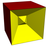 Fig 18. Cube with two intersecting pyramidal excavations
 |
Another option is also available when augmenting. The user may choose to either augment or excavate. When excavating, the second polyhedron is subtracted from the first, rather than being added. For example a cube with a square pyramid excavated from it would leave a pyramid-shaped dimple in one side of the cube. Another term, drilling, is used when the excavation leaves a hole right through the polyhedron, thus increasing the genus. Stewart [25] did much work on excavations and drilling in his fascinating self-published book. He extended Johnson's work [10] from the convex to the non convex, with some beautiful results. The hand-drawn images, however, can leave the reader a little lost unless they attempt to build some of the models themselves. As we mentioned earlier, all the Johnson solids and many of the Stewart toroids are already built-in models in Stella, and using the augmentation and excavation features most of the other Stewart toroids can be constructed, along with new ones not covered in the book. A note should be made here about how drilling works, to avoid confusion. It is not like carving up a block of wood. Take a cube and make an excavation in two opposite sides using a pyramid (J1). The height of the pyramid is greater than half the height of the cube, so the two peaks pass through each other (see figure 18). However this does not cut a hole through the model as it would when using CSG (constructive solid geometry) in a typical 3D modelling package. Instead, the geometer doesn't generally mind faces passing through each other unscathed, as demonstrated by the ancient Kepler-Poinsot polyhedra. However the geometer generally doesn't want a model with coincident faces, so any faces of the original polyhedron which coincide with any faces of the augmentation model are removed in pairs, and the surrounding edges stitched up again to leave only two faces meeting per edge. This of course includes the original face where the augmentation took place, but may include other faces too.
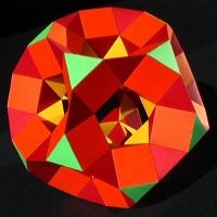 Fig 19. Drilled truncated dodecahedron
 |
One convenient side effect of this methodology is that if the user wants to undo their last augmentation, they can do it by excavating the same model again. All the new faces caused by the augmentation will line up with faces from the excavation, and are therefore removed, leaving the original model again.
Just to jump straight into the deep end, have a look at figure 19 for an example of one of the most stunning Stewart toroids from his book. This model is built into Stella, but if we wanted to make it from first principles, so to speak, we could do it as follows, using the other built-in models. Put the pentagonal cupola in memory 1, put the pentagonal antiprism in memory 2, and put the dodecahedron in memory 3. Now load up the truncated dodecahedron and select one of the decagonal faces. Excavate memory 1 from all such faces, then select the pentagonal face at the base of one of the cupolaic excavations. This time excavate memory 2 from all such faces, and select one of the new pentagonal faces. And finally, excavate memory 3 from this face. The result should be the model shown.
It should be pointed out, however, that the presence of only four memories does not limit the number of different excavations that can be made. The current model can be put into memory at any stage, and different models placed into the other memories. The original model can then be retrieved and further excavations made using the updated memories.
When there is any ambiguity about which face of the model in memory should be connected to the selected face of the model on the screen, as with the square cupola, which has two types of square faces, the user should first select the appropriate face before putting the model in memory. Regarding scale, the model in memory will be scaled up or down if required so that the faces match, so the user need not worry about this aspect.
Many new Stewart toroids can now be discovered with a bit of ingenuity (the reader is referred to Stewart's book [25] for the definitions of terms and symbols used in this paragraph). Using Stewart's terminology, an interesting new model is K5 / T5 (R5) gQ5. It is probably the most "cavernous" of the Stewart toroids that satisfies all his rules. That is, roughly speaking, it's got the biggest hole. This model can also be used as the base for a four-storey model with fewer faces than Stewart's example by further drilling the inner truncated dodecahedron. These models are not built in, but are included in an additional library of models that comes with Stella.
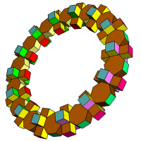 Fig 20. Toroid using only heptagons and squares
 |
Another thing Stewart investigates early in his book is whether any models of genus greater than zero can be constructed using only n-gons and one other type of polygon, for any n. Faces sharing an edge must not be coplanar. He shows how this is possible for any even value of n, but it can now be demonstrated that any odd value is also possible. For an example using n = 7, see figure 20. This model consists only of heptagons and squares, and was constructed by augmenting heptagonal prisms and cubes together. The same technique can be used for any odd value of n > 3. The n = 3 case is solved explicitly in Stewart's book, so the problem can indeed be solved for any value of n > 2.
Stewart's approach to extending the idea behind the Johnson solids from the convex to the non convex was just one approach. The main idea that the faces must be regular should probably be kept for any extension, but beyond that there are a few different directions to take. Stewart also kept the idea that faces must not intersect, and investigated several other rules. Another approach is to allow faces to intersect, but add other restrictions to limit the set. One thought is that it would be nice to find more models that have the aesthetic appeal of the uniform polyhedra. With this in mind the author considered the following additional restrictions:
- Must be locally convex. That is, the faces surrounding each vertex must loop around the vertex in the same direction (no retrograde faces spanning back the other way, but star vertices would be acceptable).
- All vertices must also be vertices of the convex hull. This is to ensure that all vertices are visible, and is a condition always met by the uniform polyhedra.
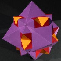 Fig 21. Augmented great cubicuboctahedron
 |
Unlike with the Johnson solids, these rules allow some models with octahedral and icosahedral symmetry. A complete enumeration would be difficult, but four new models have been found based on augmentation of the uniform polyhedra, one octahedral, and three icosahedral as follows:
- Great cubicuboctahedron. Augment square faces with square pyramids (see figure 21).
- Dodecadodecahedron. Augment pentagonal faces with pentagonal pyramids.
- Great ditrigonal dodecicosidodecahedron. Augment pentagonal faces with pentagonal pyramids.
- Snub dodecadodecahedron. Augment pentagonal faces with pentagonal pyramids.
We believe these models are new, and have not been published previously.
A polyhedron may have rotational and reflective symmetries. A rotational symmetry is an axis about which the model can be rotated (through some angle less than 360 degrees), such that it aligns exactly with its starting position. So an observer would not be able to tell that it had moved. If the minimum such angle is 360/N degrees then we call this an N-fold axis of symmetry. Similarly, a reflection symmetry is a plane in which the model can be reflected, again leaving it indistinguishable from its original position.
The collection of all such symmetries for a model is called its symmetry group. For a comprehensive beginners guide to symmetries and symmetry groups, see Cromwell [4].
7.1. Finding and showing symmetries
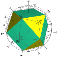 Fig 22. Cuboctahedron and its symmetries
 |
When a new model is created, either by selecting it from the built-in list, or via faceting, augmentation, or any other method, it is automatically analyzed to find its symmetries, including rotations and reflections. The name of the rotational symmetry group and associated reflection group are displayed side by side at the top of the window. The algorithm is based on Waltzman's algorithm [26], but is such that the correct symmetry group is still found for tricky cases such as compounds, or models with holes along some rotational symmetry axes. This is achieved by first finding the convex hull and its symmetries, which are then tested in full against the original polyhedron.
If using the default coloring scheme, faces of the same type are then given the same color based on the model's symmetries, and faces of different types receive different colors.
The interface allows the user to display the rotational or reflective symmetries, or both, on the screen (see figure 22). Rotational symmetries are displayed as axes through the model. A small disc with spokes is displayed at each end, the number of spokes indicating the order of rotational symmetry around that axis. For example five spokes will be shown for a 5-fold rotational symmetry axis. Axes of different order are also shown in different colors.
Reflection planes are displayed as great circles in the appropriate plane around the model. The less common central inversion and rotation-reflection types of reflection symmetry are not represented graphically, but their presence is still indicated at the top of the screen.
Rotation and reflection symmetries may also be displayed on stellation diagrams. In this case rotational symmetry axes are displayed as points where an axis intersects this facial plane. The points are displayed in the same colors as the axes in the 3D view of the model for easy cross-reference. In the case of models with hemispherical faces, that is, faces that pass through the very center of the model, only axes which lie in that plane are displayed, and they are shown as dashed lines in the appropriate color.
Reflection symmetries are displayed in the stellation diagram as dashed lines representing the intersection of the facial plane with that reflection plane. They are displayed in the same color as the great circles in the 3D view, again for easy association.
The rotational and reflective symmetry group names are actually displayed in drop-down lists, each containing the names of all possible sub-symmetry groups. The user may select a sub-symmetry group from these lists, instead of using full symmetry. Faces are then re-colored accordingly, and if symmetries are displayed, they too will be updated. For example, if we just consider rotational symmetries for the moment, 4-fold dihedral symmetry, like that of the square antiprism, is a sub-symmetry of the full octahedral symmetry group. When a cube is loaded into the program, all faces will be the same color, as they are all of the same type, and the program will indicate the octahedral symmetry group for the model. However, if the user then selects the 4-fold dihedral sub-symmetry group, then two colors will be used. One for the top and bottom face, which lie on the 4-fold axis, and another for the remaining four faces, which all lie on 2-fold axes.
A sub-group of the reflection symmetry may also be chosen. For example, start with a model of octahedral symmetry and choose the tetrahedral rotational sub-symmetry group. Now the list of available reflection types will be diagonal (like the regular tetrahedron has), horizontal (three orthogonal reflection planes), or chiral (no reflective symmetry).
 Fig 23. Tetrahedral stellation of dodecahedron
 |
Once a sub-symmetry group has been selected, it affects how stellation, faceting, and augmentation/excavation operate. Sub-symmetric stellations may now be created. Ounsted [20] gave an example of a sub-symmetric stellation of the dodecahedron, having only tetrahedral symmetry (see figure 23). In fact, the dodecahedron in particular has many interesting tetrahedral stellations. Appealing tetrahedral stellations of the icosahedron and rhombic triacontahedron have also been discovered.
Sub-symmetric facetings are also available. Here, when creating the faceted model, each facet the user has created will only be repeated over the sub-symmetry group. Most of Klitzing's faceted models [12] are sub-symmetric, so here we have an example of the usefulness of sub-symmetric facetings.
The sub-symmetry setting also has an effect when using augmentation and choosing to augment all faces of a type. Due to the sub-symmetry group, there may now be fewer faces of the same type as the selected face, so fewer augmentations will be added. Again, more interesting models can be made via this feature, such as icosahedral symmetry models being drilled tetrahedrally. Sometimes this is required in fact to avoid intersections between the models used for the excavations that would have occurred with full symmetry.
Another thing Stella allows us to do is view polyhedra morphing into their duals and back in real-time. There are five different techniques to choose from for this task. The user can drag the mouse back and forth to control the morphing. If the mouse button is released while still being dragged then the morphing continues on its own at the current rate. It should be noted that these algorithms are not guaranteed to work for every model. They work well for most uniform polyhedra (except those with infinite duals), but there are problems with some other models. We hope to rectify this soon. The five techniques are outlined below.
- Morph by sizing
 |
 |
 |
|
 |
|
 |
|
 |
| Fig 24. Morphing duals by sizing |
This is the simplest technique. Simply change from the model to its dual by shrinking the model, and growing the dual from zero size until the original model has vanished and the dual model is all that remains, at full size. As the sizing occurs the user will see the dual's vertices poke through the original model's faces, and eventually the original model's vertices will sink into the dual and vanish. The technique is simple enough to work for any model.
Each technique has a dual technique. If we imagine taking the dual of each intermediate model along the path from a polyhedron to its dual, we will get another morphing sequence that runs from the dual back to the original model. If this sequence is played in reverse, it will run from the original model to its dual again, and thus represents another possible technique. This first technique, however, is its own dual.
- Morph by truncation
|
|
 |
|
 |
|
 |
|
|
| Fig 25. Morphing duals by truncation |
From either end of the transition, the model is slowly truncated towards the midpoint. Consider a cube for example. First the tips of its vertices are truncated, then more so, past the familiar Archimedean truncated cube, until the truncations meet each other half way along the original cube's edges. Here we have the cuboctahedron. If we had started with the cube's dual, the octahedron, a similar thing would have happened, past the truncated octahedron until we again reached the cuboctahedron. This last part is played in reverse to get from the cuboctahedron to the octahedron, thus completing the transition from cube to octahedron. It may be surprising to discover that this technique works quite well for any uniform polyhedron, even though faces intersect, and indeed it works very well for most Stewart toroids, which is a sight to behold!
The definition of exactly what happens must be a bit more precise for models such as the Johnson solids. Here's a better way to think of this transition happening: start with the original polyhedron and imagine its dual is already there, but invisible, and scaled up big enough to enclose it. Now as we head towards the midpoint, shrink the dual to its normal size. As it shrinks, vertices of the original model are truncated by their corresponding faces in the shrinking dual. At the halfway point, the dual stops shrinking and the original model starts growing, until all of its faces are beyond their corresponding dual vertices.
- Morph by augmentation
|
|
 |
|
 |
|
 |
|
|
| Fig 26. Morphing duals by augmentation |
This is the dual transition to the previous one. Rather than vertices being truncated, faces are augmented with pyramids. The previous technique introduced a new face for each vertex, and this one introduces a new vertex for each face. Consider a cube. Start by building very shallow square pyramids on each face, then slowly grow them in height, past the tetrakis-hexahedron (dual of the truncated octahedron) and on until triangles from adjacent pyramids become coplanar, giving us the rhombic dodecahedron (dual of the cuboctahedron). Now consider starting from the cube's dual, the octahedron. Build shallow triangular pyramids on each face and grow their height slowly, past the triakis-octahedron (dual of the truncated cube) and on again to the rhombic dodecahedron. Play this last part in reverse to get from the rhombic dodecahedron to the octahedron, which completes the transition from cube to octahedron. Notice how all the models we passed along the way were duals of those we past using the previous technique, but in reverse order?
The technique does not work perfectly for some non-uniform models. With some Johnson solids for example, the apex of the pyramid starts outside the face at its shallowest, which causes problems. We plan to generalize our algorithm further to account for these cases.
- Morph with rectangles
|
|
 |
|
 |
|
 |
|
|
| Fig 27. Morphing duals with rectangles |
This technique was described by Lalvani [13], who dedicated a whole book to it! It is quite straightforward, and seems to work well for any model, including uniforms, Johnson solids, and even Stewart toroids! Faces of the original model are shrunk, and faces from the dual start to appear at the original model's vertices. Then rectangles are used to fill the gaps between the two. An example will help here, so again, let's start with a cube. The vertices are truncated and the edges bevelled to leave a small triangle where each vertex was, and a long thin rectangle where each edge was. Continuing to cut deeper we get to the rhombicuboctahedron, which is the halfway point. Note that the original square faces are shrinking, and the dual triangle faces are growing, but neither one ever changes orientation. The rectangles between start long and thin, get fatter until they are squares, and then continue until they are long and thin in the opposite way.
- Morph by tilting quads
|
|
 |
|
 |
|
 |
|
|
| Fig 28. Morphing duals by tilting quads |
Finally, we have the dual of the previous technique. During the previous transition, all vertices have a valency of four, with one face from the original model, one face from the dual model, and two rectangles surrounding them. So, during this dual technique, all the faces will be quadrilaterals. Starting with a cube, notice that the midpoints of the edges coincide with the midpoints of the dual octahedron's edges. Take two consecutive edges in one of the square faces and connect their midpoints to the center of the face, and to the intermediate vertex to form a quadrilateral. Holding the edge midpoints still, the quadrilateral can be tilted (and distorted, but kept planar) so that the point at the face center extends out towards the corresponding dual vertex, and the point that started at a vertex heads in towards the center of its corresponding dual face. When they reach these points, the quadrilaterals meeting at one of the original vertices become coplanar and form the dual face. Note that at the halfway point we find the strombic icositetrahedron, dual of the halfway point using the previous technique, the rhombicuboctahedron.
In the general case, it is not always the midpoints of the edges that we are interested in, but rather the point found by dropping a perpendicular onto the edge from the center of the model. Note also that for non-uniform cases, the edge-points may not coincide between the duals, but a line through corresponding pairs should go through the center of the model. In this case the edge-points need to be interpolated too, rather than being held still.
A number of other features are worth a mention here.
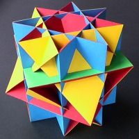 Fig 29. Pseudo great rhombicuboctahedron
 |
- Pseudo-uniform polyhedra can be made. These are polyhedra that are locally uniform only, that is, each vertex is surrounded identically by faces, but does not share the same relationship to the solid as a whole. As it turns out there are only two such models. One is also known for being a Johnson solid (J37, the elongated square gyrobicupola). Each vertex is surrounded by a triangle and three squares. It is like the Archimedean rhombicuboctahedron with one of its square cupola caps twisted 45 degrees. The other pseudo-uniform polyhedron is the lesser known, and was described by Jones [11] (see figure 29). It is in fact isomorphic to J37, that is, it has the same topology, and is a variation of the uniform great rhombicuboctahedron. Again, a cap must be twisted, but it is somewhat harder to visualise now that all the faces intersect!
- The convex hull of any model can be generated.
- There is a measurement mode where the user can click on any two vertices of a model to find out the distance between them.
- Stella has a spring network relaxation system built in, which was used to generate the coordinates for the Johnson solids and some of the Stewart toroids. Many thanks go to Jim McNeill [15] for advice on achieving this. His own system is available from his web site. We still have some work to do on the spring system to make it more useful and friendly for the end-user, but for now we are satisfied that it has provided us with the coordinates needed for a variety of models. The basic idea is to create a spring for each edge. A spring has a rest length of one, say, which represents all edges having the same length. Vertices start off at random positions, and then the springs try to push or pull the vertices at each end to achieve the desired length. This process repeats for many iterations until the springs are all very close to their desired lengths. In practice, the spring models often form knots and isomorphs of the desired models, so extra springs are inserted in various ways and of different lengths to give the system a better chance of finding the correct model. Stella's interface does allow the user to specify their own faces for use with the spring system, but as we said, this is an area that needs further work.
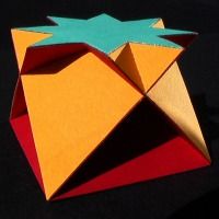 Fig 30. Crossed square cupola
 |
Cupolae, cuploids, and cupolaic blends of arbitrary base can all be created in Stella (see figure 30 for an example). The user selects one of these three types of polyhedron and is prompted to enter the base type. The spring system is then employed internally to construct the model in such a way that success is guaranteed (it won't find knots). These are examples of regular-faced polyhedra, where the vertices fall into two parallel planes. A few convex cupolae exist, but otherwise the models are all non convex and self-intersecting. They are an interesting class of polyhedron, with pyramidal symmetry.- There are advanced coloring options for automatically coloring the faces of models the way the user wants. Alternatively, the user can manually select faces and change their colors. There is also an option to automatically color compounds, with one color per component.
- Models may be exported to a number of popular 3D formats, including DXF, POV for the POV-Ray ray-tracing program, VRML for use on web sites, OBJ for Alias|Wavefront, and OFF, a simple text format which can be easily parsed for other applications.
- In addition to exporting via common 3D formats, models may also be saved and reloaded in Stella's own file format, which also remembers the current window layout and other information. A library of over a hundred extra models is included with Stella, using this format. This includes all the models referred to in this paper and many more.
10. Conclusion
We have presented a computer program called Great Stella, which allows the user to navigate their way through the trillions of fascinating polyhedra available. A wide range of tools including stellation, faceting, augmentation, excavation and drilling ensure the user will never run out of interesting avenues to explore. Many new and intriguing polyhedra have already been discovered, and many old favorites rediscovered.
Nets for any model may be printed out, with parts being grouped by color if required, for printing directly onto colored paper. What was traditionally a hobby requiring a high level of mathematics may now be pursued by anyone. Models may be constructed much faster without the need to manually perform the many initial calculations. Designing and drafting the nets is now also a thing of the past, with this too being automated. The model-maker may decide for themselves how deep they wish to go into the theory involved. The geometric theory is still there for those interested, but others can now make polyhedra purely for their aesthetic appeal.
The program is available from the author's web site [27].
Acknowledgements
The author would like to thank Fiona Clarke, Peter Messer, Guy Inchbald, and Ulrich Mikloweit for their useful comments regarding this paper.
References
- Coxeter, H. S. M., Du Val, P., Flather, H. T., J.F. Petrie, "The Fifty-Nine Icosahedra", University of Toronto Press, 1938.
- Coxeter, H. S. M., Longuet-Higgins, M. S., Miller, J. C. P. "Uniform Polyhedra", Philosophical Transactions of the Royal Society of London Series A, Vol. 246, pp. 401-450, 1954.
- Coxeter, H. S. M. "Regular Polytopes", Macmillan, 1963. (Dover reprint, 1973).
- Cromwell, P. R. "Polyhedra", Cambridge, 1997.
- Cundy, H. M., Wenninger, M. J. "A compound of five dodecahedra", Mathematical Gazette, Vol. 60, pp. 216-218, 1976.
- Ede, J. D. "Rhombic Triacontahedra", Mathematical Gazette, Vol. 42, pp. 98-100, 1958.
- Fleurent, G. M. "Symmetry and Polyhedral Stellation Ia & Ib", Computers and Mathematics with Applications, Vol. 17, No. 1-3, pp. 167-193, 1989.
- Hudson, J. L., Kingston, J. G. "Stellating Polyhedra", The Mathematical Intelligencer, Vol. 10, No. 3, pp. 50-61, 1988.
- Inchbald, G. "Towards stellating the icosahedron and faceting the dodecahedron", Symmetry: Culture and Science, elsewhere in this issue, 2002.
- Johnson, N. W. "Convex Solids with Regular Faces", Canadian Journal of Mathematics, Vol. 18, 1966, pp. 169-200.
- Jones, R. H. "The pseudo-great rhombicuboctahedron", Mathematical Scientist, Vol. 19, No. 1, June, 1994, pp. 60-63.
- Klitzing, R. "Facetings of Uniform Polyhedra", http://www.polyedergarten.de/e_Klintro.htm
- Lalvani, H. "Transpolyhedra: Dual Transformations by Explosion-Implosion", Published by the author, 1977.
- Luke, D. "Stellations of the Rhombic Dodecahedron", Mathematical Gazette, Vol. 41, pp. 189-194, 1957.
- McNeill, J. "Hedron", software program, http://web.ukonline.co.uk/polyhedra/hedron.html
- Messer, P. W., Wenninger, M. J. "Symmetry and Polyhedral Stellation II", Computers and Mathematics with Applications, Vol. 17, No. 1-3, pp. 195-201, 1989.
- Messer, P. W. "Stellations of the Rhombic Triacontahedron and Beyond", Structural Topology 21, pp. 25-46, 1995.
- Mikloweit, U. "Polyedergarten", http://www.polyedergarten.de
- Norman, A. C., Smith, A. "Computer Drawings of Compounds of Star Polyhedra", Mathematical Gazette, Vol. 57, pp. 303-306, 1973.
- Ounsted, J. "An Unfamiliar Dodecahedron", Mathematics Teaching, Vol. 83, pp. 46-47, 1978.
- Pawley, G. S. "The 227 Triacontahedra", Geometriae Dedicata, Vol 4, pp. 221-232, 1975.
- Skilling, J. "The Complete Set of Uniform Polyhedra", Philosophical Transactions of the Royal Society of London Series A, Vol. 278, pp. 111-135, 1975.
- Smith, A. "Stellations of the Triakis Tetrahedron", Mathematical Gazette, Vol. 49, pp. 135-143, 1965.
- Smith, A. "Some Regular Compounds of Star-Polyhedra", Mathematical Gazette, Vol. 57, pp. 39-46, 1973.
- Stewart, Professor B. M. "Adventures Among the Toroids", Published by the author, 1970. Revised second edition published 1980.
- Waltzman, R., "Geometric Problem Solving By Machine Visualization", Proceedings of the Image Understanding Workshop (IUW), pp. 353-354, 1989.
- Webb, R. "Great Stella 2.0", software program, 2002, available from http://www.software3d.com/Stella.html or search for "great stella", at http://www.google.com
- Wenninger, M. J. "Polyhedron Models", Cambridge University Press, 1971.
- Wenninger, M. J. "Dual Models", Cambridge University Press, 1983.
Original location of this paper: https://www.software3d.com/PolyNav/PolyNavigator.html